Calculator Help: Statistics

The calculator used in the making of this post is a TI-84 Plus Silver Edition graphing calculator. The instructions here can be used for other graphing calculators, but please note that keys/menus may be in different locations on different calculators.

Today we are going to learn how to use a graphing calculator to work with statistics. Statistics is used to generalize a specific set of data and find patterns and correlations between things. We will be using the STAT button (green) on the calculator to access most of the menus we need. We will also need the STAT PLOT menu found by pressing 2nd, then Y= (yellow). And the LIST menu, which is found by pressing 2nd, STAT (green).

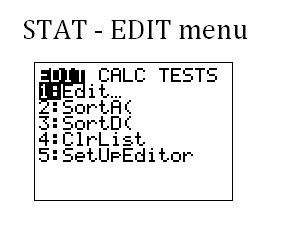
The first menu that you see when you press STAT is the STAT-EDIT menu (below). The first option (1: Edit...) allows you to edit the stat lists (more about that later); the second option (2: SortA( ) will sort a list in ascending order; the third option (3: SortD( ) will sort a list in descending order; the fourth option (4: ClrList) allows you to quickly clear one or more lists; and the fifth option (5: SetUpEditor) allows you to change the order in which the lists appear in the edit screen.

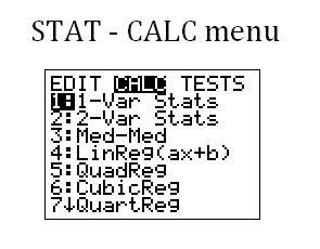
Arrow to the right and you will see the STAT-CALC menu (below). The first two options allow you to obtain statistical data on one or two lists; the third options calculates a median-median line (you probably won't use this one); and all other options allow you to fit regression lines of various types. You will probably mostly use 2: 2-Var Stats and 4: LinReg (ax + b) for a basic algebra course. 

Press 2nd, STAT to open the LIST menu (not pictured). The first menu you see is the LIST-NAMES menu. Here, you can see a list of all lists that you've created. If you've named them, their names will appear here. Arrow to the right to see the LIST-OPS menu, a list of various operations you can perform on lists. And if you arrow to the right again, you will see the LIST-MATH menu which shows you various math operations you can perform on a list, such as finding the mean or median.

You probably won't use this LIST menu in a basic algebra course, but you should play around with it a little because it does contain some helpful things. Use your user manual to learn more about this LIST menu.

We will also be using the STAT PLOT menu, which can be found by pressing 2nd, Y= (below). Here you will see a list of 4 stat plots available for you to use. At first, they will probably all be turned off, but we will learn how to use them later. Press ENTER on one of the stat plots to see options for that plot--you can turn the plot on or off, change the type of graph it will use, change the lists that the X and Y values will come from, and change the type of mark the calculator will place for each data point.

The best way to learn how to use these STAT operations is to work through an example. Consider the following situation. A student is studying ant behavior by putting a number of candies out by an ant hill, and then counting how many ants are attracted to the candy. Her data follows:

If you are given a word problem, the first step is to identify the variables. The independent variable (x) is the variable that the observer alters. In this case, the student is changing the number of candies, so the number of candies will be our x-values. The dependent variable (y) is the result of the change in the independent variable. In our case, the number of ants changes as a result of the change in the number of candies, so the number of ants will be our y-values.

In order to statistically study the correlation between the number of candies and the number of ants, we need to first input these data values into lists.

How to Input Statistical Data in Lists

1. Open the STAT menu. Choose option 1: Edit...

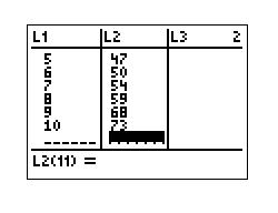
2. Input the x-values into L1 and the y-values into L2. Type in the first x-value and press ENTER to move down the list. When all x-values have been entered, press the RIGHT arrow key and then enter the y-values the same way into L2. Below is an image of what you will see when you've pressed ENTER on the final y-value.

How to View Statistic Plots

1. After entering the data in the desired lists, choose 2nd, Y= to open the STAT PLOT menu. Press ENTER on the first plot to see options. Press ENTER on "On" to turn this plot on; choose the first type of graph (probably is already selected); be sure that L1 is chosen for the Xlist and L2 is chosen for the Ylist; and choose the first "box" mark. If your Xlist or Ylist values are incorrect, you can enter the correct values by pressing 2nd, then a number on the keypad that corresponds to the list you want. In blue above the numbers on the keypad, you should see "L1," "L2," etc. Below is how your screen should look when all options are chosen.

2. Press Y= and clear any functions that appear in the y-slots. Then press WINDOW to alter the window to show all data points. The domain in our example is (1, 10) so set Xmin to 0 and Xmax to 11 (so that we can see all the points). Our range is (15, 73) so set Ymin to 0 and Ymax to 80 (so that we can see all points). I've chosen my Xscl to be 1 and my Yscl to be 2 so that the y-axis is not too crowded with points. Here is an image of the WINDOW screen after edits have been made.

3. Press GRAPH to see the stat plot.

After you've plotted the data, you may wish to find out some information about the statistics you've entered. In a plot of two variables, as in our example, you will use the 2-variable stats.

How to View 2-Variable Stats

1. After inputting data (it doesn't need to be plotted in a graph), open the STAT menu, then arrow to the right to the STAT-CALC menu. Choose option 2: 2-Var Stats.

2. Enter the lists you used in the Xlist and Ylist options. In our example, we want these to be L1 and L2, respectively. If they are incorrect on your screen, change them by pressing 2nd, then a number on the keypad (1-6). Ignore the FreqList: option unless your instructor tells you how to use it. Then press ENTER on Calculate to see the results.

Here, you can see all sorts of information about the data you entered. You are given all sorts of statistics. Here is a list of the variables you see and what they stand for, and the values for our example:

Looking at the graph of the data points in this example, we can see that it appears to form an almost linear trend (points form a nearly straight line). We can use the calculator to easily fit a linear best-fit line to our data points. There are many types of regression lines, but we will look at a linear regression for our example.

How to View a Regression Line

1. After inputting the data and plotting the graph (plotting is optional, but recommended), open the STAT menu and arrow to the right to see the STAT-CALC menu. Choose option 4: LinReg (ax + b).

2. Set the Xlist and Ylist to the appropriate list names (our example uses L1 and L2, respectively). Ignore the FregList option. The next option is asking if you want the calculator to store the linear regression equation in a y= value. This will allow you to easily graph the equation it gives you without having to manually enter it into the y= line. We want to do this, so with the cursor on this line, press VARS (to the left of the CLEAR button) and then arrow to the right to the Y-VARS menu. Choose option 1: Function... and then choose option 1: Y1. We are telling the calculator to store the regression equation in the first function line in the Y= menu.

3. Press ENTER on Calculate to see the results.

Here, you are given the equation format, the slope (a), and the y-intercept (b) of the regression equation. Press Y= and you will see that the equation has been entered into the first function line. Now press GRAPH to see the regression line plotted over top of the data points.

Wasn't that just too easy?

After using the statistics functions, you may wish to clear the lists you've used. To do so, open the STAT menu and choose option 4: ClrList from the STAT-EDIT menu. Then enter the lists you wish you clear, separating multiple lists by commas. Then press ENTER.

You may also want to turn all stat plots off so that you don't forget to do this when graphing functions later on. To do this easily, open the STAT PLOT menu by pressing 2nd, then Y= and choose option 4: PlotsOff. Press ENTER on the home screen and the calculator will turn all stat plots off for you.

I hope this post has helped you learn how to use the stat options on your graphing calculator. It is really easy, once you know your way around the menus.

Calculator Help: Input Functions

CLICK HERE to view the YouTube video that corresponds to this post.

This post is the first in a series I’m doing that will help you use your graphing calculator. The calculator I’m using for demonstration is a TI-84 Plus Silver Edition graphing calculator. These instructions apply to any TI-83 or TI-84 calculator. If you are using an older model, such as a TI-82, the steps are essentially the same, but some buttons/menus will be in different places. If you are using a newer/higher model, such as the TI-89, most of the buttons/menus will be in the same place, but your screen may look different than mine.

Also, I have the newest operating system on my calculator. The new operating system differs from the old in that it handles fractions more easily. If you are interested in downloading the new OS to your calculator, you need to have the TI Connect software and a mini-USB to USB cable. Your calculator, if bought new, should have a CD with it and a cable. If you don’t have the CD, the software can be downloaded from the web and you can use any mini-USB to USB cable you may have around.

It is not necessary to have the newest OS on your calculator for my demonstration purposes. I just wanted to explain why my calculator screen may look a bit different than yours.

Today’s lesson will cover how to graph functions. We will input functions into the calculator and adjust the window settings to see the function in the GRAPH screen.

For this explanation, we will be using the Y= menu, the WINDOW menu, and the GRAPH screen. You can get to these menus and screens via the buttons circled in yellow (Y=), red (WINDOW), and green (GRAPH). We will also use the ZOOM key, which is to the right of the WINDOW key (not circled) and the variable key, which is to the right of the ALPHA key (circled in a later photo).

Take a minute to go through these menus and get familiar with them.

When inputting a function into the calculator, you need to solve for y first. That is, the calculator only understands functions if they begin with “y=.” Your function may use other names for y, such as f(x), g(x) or something similar. Simply replace this f(x) or g(x) or whatever with y. Also, your function may use some other variable than x, so you can simply replace that variable with x because the calculator only recognizes the variable x in a normal function.

Before going over the steps to input a function into your calculator, there are two things you need to check first. Open the Y= menu and check these two things:

1.  Is there a function (or more) in any of the Y slots? If there is, arrow to that slot and press the CLEAR button to erase it.

2.  Is one of the Plots at the top of the screen highlighted? If one is (or more are) highlighted, arrow up and over to it and press ENTER to disable it. (To check this on the TI-82, you will have to press 2nd, then Y=, and then choose option 4: PlotsOff, then ENTER on the home screen to turn all stat plots off.)

How to Input a Function

1.  Solve the equation for y if it is not already in the correct form.

2.  Open the Y= menu and type the equation into the first entry, beginning after the equals sign. Fractions must be input between parentheses. The variable x is entered using the variable key (circled in red on the calculator image below.)

3.  Press GRAPH to graph the function. If you cannot see this function in your screen, press ZOOM, and then choose option 6: ZStandard to return your window to the standard window dimensions. We will discuss how to alter the window for other functions later.

The term window refers to the viewable area of the graph screen. The standard window is x: (-10, 10) and y: (-10, 10), both with scale set to 1. This means that in the standard window, you can see from -10 to 10 on the x-axis and from -10 to 10 on the y-axis and there is a tick mark for every 1 unit. For many functions, this graphing window is acceptable and all important aspects of the graph will be shown. For others, however, this window may not show some important characteristics of the graph, and you will have to manually adjust the window.

Graph the following function using the steps above.

You should see the image below in your GRAPH screen.

Notice that the function is quadratic with a y-intercept at -32. The standard window, however, is not large enough to show this y-intercept. Therefore, we must adjust it. Use this graph to follow the steps below and adjust the window to see the y-intercept.

How to Adjust the Graphing Window

1.  Graph the function.

2. If you already know which pieces of the graph are not showing, you can skip this step. If you are not sure which part of the window needs to be altered, press ZOOM and then choose option 0: ZoomFit. This should allow you to see the important parts of the graph that were previously hidden. However, you should still adjust the window further to allow for a clearer picture.

3. We know that the function we’ve graphed has a y-intercept at -32, so our minimum y-value shown must be at least -32 for us to see the whole graph. Press WINDOW and arrow down to Ymin and input -50 here. Our window is now x: (-10, 10), y: (-50, 10), and both scales are 1. With our y range so large, however, the axis will be very cluttered with a y scale of 1. So let’s change Yscl to 10 so that there will be a tick mark every 10 units on the y-axis.

4. Press GRAPH again to view the changes we made. The graph is now clearer, easier to read, and the important minimum value is easy to see.

You may need to adjust the window a little at a time until you are satisfied with the graph you see. It may be helpful to manually find the y-intercept first, so that you can get an idea of where the function crosses the y-axis. You can also manually find the x-intercepts for the same reason.

Adjusting the window is not a set process because it works differently for every function. You will need to play with it by making small changes and returning to the graph to view them.

I hope this post has helped you feel more comfortable with inputting functions into a calculator for graphing.

Trigonometry: Angles and Arcs, Part 2

CLICK HERE to view the YouTube video that corresponds to this post.

This is the second part of a set of posts dealing with angles and arcs in Trigonometry. In the first part, I covered some definitions pertaining to angles, how to find complements and supplements of given angles, how to find angles coterminal to a given angle, and how to convert between DMS notation and decimal degrees. If you haven't read that post, I highly suggest you do, and you can find it by following this link.

In this part, I will cover arcs and angles measured in radians. We will look at the formula for calculating arc length, as well as how to convert between radians and degrees. At the end, I will give you steps for solving application problems.

First, let's answer a question that I am asked frequently: "What is a radian?" This stumps many students because, prior to taking Trigonometry, they probably never heard the word.

A radian is the measure of an angle formed when an arc of length r is subtended on a circle of radius r. This means that if you have a circle of any radius and you measure an arc length equal to that radius, then the angle formed by that arc length is defined as exactly 1 radian.

There are π (pi) radians in a half circle and 2π radians in a full circle. Therefore, π radians correspond to 180 degrees and 2 π radians correspond to 360 degrees.

An important element of Trigonometry is converting between radians and degrees. These are the two most commonly used units of measure for angles. All you need to remember is the conversion factor I just gave you (and also shown in the blue box below).

How to Convert Between Radians and Degrees

Let's try some example problems. In the problems below, I've boxed the angle we are converting in blue, the conversion factor we are using in green, and the answers in red. After multiplying by the correct conversion factor, you simply need to reduce fractions and simplify as much as possible. A common error students make is to use 2 π radians instead of just π radians in the conversion factor; avoid this by memorizing the conversion factor properly.

You can also use your calculator to convert between radians and degrees, though it is not very efficient to do so. In the beginning, you can use this method to check your answers for converting between degrees and radians.

How to Use Your Calculator to Convert Between Degrees and Radians

 Step 1: Make sure your calculator is in the mode corresponding to the unit you are converting TO. To check what mode your calculator is in, press the MODE key (next to the 2ND key). In this menu, about 3 options down, you will see RADIAN DEGREE, with one of these highlighted (look at red box in images below). If the one highlighted is not the unit you are converting TO, arrow down to this row and then arrow over and press ENTER on the unit you want to choose. Below you can see the menu options. In my MODE menu on the left, RADIAN is highlighted, which indicates that my calculator is in RADIAN mode. I can only convert FROM degrees TO radians in this mode. If I want to convert FROM radians TO degrees, I have to change it to degree mode, as shown on the right.

Step 2: Press 2ND then MODE to exit the MODE menu. Input the angle you wish to convert. To input DEGREES, press 2ND then APPS to enter the ANGLE menu. Choose option 1 for the degree symbol (boxed in red below). To input RADIANS, press 2ND then APPS to enter the ANGLE menu and choose option 3 for the radians symbol (boxed in blue below).

Step 3: Press ENTER to tell your calculator to make the conversion.

There are two things you need to note when using your calculator to make this conversion.

1. For fractional radian measures, you MUST input the fraction in parentheses before inserting the radians symbol. In the image below, you can see that if I do not put parentheses around the fraction, the computer does not arrive at the correct answer! (See below)

2. When converting TO radians, the calculator will not show you the answer in terms of π. It will, instead, give you a decimal approximation. Do not use this decimal as your answer. Instead, convert it back into a fraction. First, divide by π and convert into a fraction (press MATH and choose 1: >FRAC to have it convert the fraction for you). Then simply multiply by π in the numerator to get your final converted answer.

I hope by now you can see that using the calculator to work through conversions is definitely not as quick as simply multiplying by the conversion factor!

Next, let's look at arc length. Arc length is the linear distance of a circle. Imagine a very large circle on the ground. If you were to walk along the circumference of this circle, you'd be walking an arc. To calculate this linear arc length, you use the arc length formula. Note that the angle measure MUST be in radians when using this formula. If the angle is not given in radians, you must convert it before using the angle measure.

Here is an example problem for finding the arc length.

Similarly, you can work problems with other variables given. If you are given arc length and radius, you can solve for the angle. If you are given arc length and angle, you can solve for the radius of the circle.

Application problems dealing with arc length often confuse students, but they are not difficult to work. Pulleys are often the stage for arc length questions. Let's work an example together.

How to Solve Arc Length Application Problems
Step 1: Draw a picture to represent the situation at hand, if one is not given already. Consider my drawing in the example. I have a larger pulley connected to a smaller pulley. I identified the larger pulley as the first pulley. Use subscripts to distinguish between the parts of one pulley versus another.

Step 2: Label all variables on the image, and then list all known variables. In my example, I am given the radius of each pulley and the angle measure of the larger pulley. The question is asking what angle the smaller pulley makes when the larger makes one revolution. Remember that in the arc length formula, the angle must be in radians, so I have quickly converted 1 revolution into radians. One revolution is equal to 2π radians.

Step 3: Set up equations for the variables you've labeled. In the example, I've written the equations for the arc lengths of each individual pulley.

Step 4: Make a connection between equations if you have more than one. Here is where students get thrown off. When two pulleys are connected by a belt, the arc length that one pulley describes is the same as the arc length the other pulley describes. The difference lies in the angles they create. The smaller pulley will subtend the larger angle. In order for the belt to move the same distance along the smaller pulley, it has to make a larger angle because the pulley is smaller. Think of this: there are two bicycles. One has tires with smaller diameters than the other bicycle. If you were going to ride one a long distance, which would you choose? You should choose the one with larger tires. Larger tires mean you do less pedaling because in an equal number of revolutions (pedals), a larger tire is going to cover more ground (it has a larger circumference). The pulleys work similarly. So set up the arc lengths equal to each other and plug in the equations.

Step 5: Before plugging in known values, solve for the unknown variable. Then, plug in known values and perform all necessary calculations. Here, you want to leave radians in terms of π. The question asks you to give the answer in terms of radians and degrees. After finding the answer in terms of radians, convert your answer into degrees.

This concludes our look at angles and arcs.

Site Update

I wanted to post a quick update to share my plans for this site and upcoming topics I am working on. I still need to finish the video for the second part of the Angles and Arcs posts--I have the post complete, but am just beginning the video. I'd love to get that up later today or tomorrow.

I have a long list of topics I'd like to do and am trying to decide on the order. I have some Calculus topics in mind that I think should be done first, and then a few more Trigonometry topics. After that, I hope to work in some calculator help videos/posts.

When tutoring, I get a lot of questions about how to use a graphing calculator. Many non-traditional students or people who have recently moved from another country, may not have used graphing calculators in middle and high school. High school and college instructors tend to assume that students know the basics of how to use the calculator and often rush through explanations, thinking they are a waste of time. This leaves many people in the dark. Not knowing how to use the calculator can cost you points on an exam because (1) you don't know how to check your computations, (2) you are doing more complicated calculations by hand, which increases the chance of error, and (3) some questions require the use of a calculator and not knowing how to use the calculator means you don't know how to do those questions.

So that's where I'm hoping to go from here. I'm aiming for two videos/posts each week, but with school and tutoring and life, it may not always be possible. Keep checking for updates. You can enter an email address at the bottom of this page to receive email updates when I post something new. Also, you can subscribe to my YouTube channel (search for the user itsvictoria08) to receive updates there when I post new videos. I always link the videos and posts together. I link the title of the blog post to the video, and below the video on YouTube, I include the link to the blog post.

If you have any comments, I'd love to hear them. If there are specific topics you'd like me to cover or if there's a subject you'd like discussed, leave a comment on this post or any other post.

Trigonometry: Angles and Arcs, Part 1

CLICK HERE to view the YouTube video that corresponds to this post.

Please note that all calculator keypad instructions are intended for TI-83 through TI-84 Plus Silver Edition graphing calculators. Refer to your instruction manual to find specific keys for any other calculator.

This is part one of two posts that deal with angles and arcs. In this segment, I will cover some definitions pertaining to angles, how to find complementary and supplementary angles to a given angle, finding coterminal angles to a given angle, and converting between DMS notation and decimal degrees.

To begin this discussion, let's review some definitions pertaining to angles.

A straight angle is an angle that measures 180 degrees. A right angle is an angle that measures 90 degrees. An acute angle is an angle that measures between 0 and 90 degrees. And an obtuse angle is an angle that measures between 90 and 180 degrees. A quadrantal angle is an angle which has a terminal side on an axis line. Non-quadrantal angles can be identified by their quadrant number.

Two positive angles are said to be complementary if their sum is equal to 90 degrees. And two positive angles are called supplementary if their sum is 180 degrees.

First, we will discuss how to find a complementary or supplementary angle to a given angle. If you are given an angle, subtract it from 90 degrees to find its complement and subtract it from 180 degrees to find its supplement. Below are a few examples.

An angle is coterminal to a given angle if it contains only the addition of an integer multiple of 360 degrees. For example, the angles 45 degrees and 1170 degrees are coterminal because 1170 = 45 + 360(2). You may be asked to find an angle that is coterminal to a given angle. You only need to follow these easy steps to answer a question like this.

How to Find a Coterminal Angle
Step 1: Divide the given angle by 360 degrees. If the answer is positive, subtract whatever whole number you obtain from this. If the answer is negative, add subtract the whole number (including the sign!) minus 1. That is, if –n.kkk is the number, you will subtract (-n – 1) from the number. See example below for more clarification.
Step 2: Multiply this answer by 360 degrees to obtain the angle less than 360 degrees that is coterminal with the given angle. Two examples are below.

All of this can be accomplished very easily in your calculator. Input the given angle and divide by 360. If you then hit plus or minus, it will bring down the previous answer automatically. Here is how the screen looks.

The green, boxed items are what I manually typed into the calculator. Each "Ans" was automatically entered by the calculator when I hit the next operations key. The red boxed value would be my answer.

There are two ways to represent angle measures. The first is decimal degrees, as you probably are used to. These are angles such as 27.2 degrees or 108.3 degrees. Another way to represent angles is in DMS (Degrees, Minutes, and Seconds).

Just as there are 60 seconds in a minute when discussing time, there are 60 seconds in one minute when discussing angle measures. And, degrees work similar to hours in that there are 60 minutes in one degree. Therefore, there are 3600 seconds in one degree. These conversion factors will allow you to interconvert between these two angle representations. I will first show you how to do this manually, then will show you the "shortcut" by using your calculator's DMS conversion tool.

How to Convert FROM DMS TO Decimal Degrees
Step 1: Write the degrees, minutes, and seconds as a sum.
Step 2: Leave the degree term as is. Multiply the minutes term by the minutes-degrees conversion factor. Multiply the seconds term by the seconds-degrees conversion factor.
Step 3: Add.

How to Convert FROM Decimal Degrees TO DMS
Step 1: Split at the decimal point and write as whole degrees plus partial degrees.
Step 2: Multiply the partial degrees by the degrees-minutes conversion factor.
Step 3: If this is a whole number, then tack 0'' to the end of your answer. If it is a decimal answer, split it at the decimal point and write as whole minutes plus partial minutes.
Step 4: Multiply the partial minutes by the minutes-seconds conversion factor.
Step 5: Rewrite your answer without the plus signs.

It is important for you to know how to manually convert between decimal degrees and DMS, but your calculator provides a shortcut. Locate the ANGLE key on your calculator (this is the same as the APPS key which has different-colored lettering on it). To get into the ANGLE menu, hit 2ND, then APPS. In the ANGLE menu, you will find various items pertaining to angle measures. The ones we are interested right now are numbers 1 through 4. Number 1 allows you to enter the degree sign into your calculator; number 2 allows you to enter; number 3 allows you to enter radians into your calculator (to be dealt with in another post); and number 4 is what you use to instruct your calculator to convert into DMS form. To type the seconds symbol into your calculator, press ALPHA then the PLUS key.

First, make sure your calculator is in degree mode. To do so, press the MODE key (to the right of the 2ND key) and arrow down until you see RADIAN DEGREE. Ensure that DEGREE is highlighted black. If it is, press 2ND then MODE to return to the home screen. If it is not highlighted, arrow down to RADIAN, then arrow to the right to DEGREE, and then press ENTER. Press 2ND then MODE to exit the mode menu.

How to Use the Calculator to Convert TO DMS Form
Step 1: With your calculator in DEGREE MODE, type in the decimal degree form of the angle measure you wish to convert INTO DMS form.
Step 2: Open the ANGLE menu by pressing 2ND then APPS.
Step 3: In this menu, arrow down to option 4: >DMS and press ENTER (or simply press the number 4 on the keypad).
Step 4: Press ENTER to instruct the calculator to make the conversion for you. The angle measure in DMS will appear, rounded to the nearest whole second.

Here is what the calculator screen will look like.

How to Use the Calculator to Convert FROM DMS Form
Step 1: With your calculator in DEGREE MODE, input the angle measure in DMS form into the home screen. Type in the degree value, then open the ANGLE menu (2ND, APPS) and choose option 1: degrees. Then type in the minute value, open the ANGLE menu and choose option 2: minutes. Finally, type in the second value and press ALPHA (below the 2ND key) and then the PLUS key to input the seconds symbol.
Step 2: Press ENTER to return the angle measure in decimal degree form.
Here is what the calculator screen will look like. When reporting your answer, round according to the instructions given for your problem. If no rounding instructions are given, round to the hundredth (two decimal places) degree. (In the screen shot below, the reported answer would actually be 35.26 because the 5 would be rounded up.)

In part 2, we will look at radians and arc lengths.

Trigonometry: Proving Trigonometric Identities

**Notice:** This post was updated on March 10, 2015 to reflect a correction in the Trigonometric Identities image. The accompanying Google Document was also corrected, as was the link to that Document. If you downloaded the Google Document before 03/10/2015, please re-visit this link and download the new version. Thank you, and sorry for the inconvenience.

CLICK HERE to view the YouTube video that corresponds to this post.
Identity problems are probably the toughest part of Trigonometry for most people. They can look scary and huge and daunting, and many students become overwhelmed at just the sight of them. I hope that this post will make you less fearful of identity problems.

The first thing to address is that you need to know the trig identities. Just knowing these will make the problems half as challenging. The best way to learn them is to use them. Have a sheet with all of the identities listed (so that you don't have to flip through your book) and use this sheet only when you need it. If you think you know the identity to use, go ahead and use it and see what you get. Use your "cheat sheet" as a safety net, not as a life preserver.

I've created a small list of the main identities (reciprocal, Pythagorean, sum/difference, double-angle, and half-angle) in a document that you can print for free. You can then fold the page in half (or cut it) and keep it in your notebook as a handy reference card. You can view/print the page by following this link to the Google Document (opens in new window). Here it is below as an image for reference in this post.

The second thing you need to do is find out which identities you are required to have memorized for your test/exam. Ask your instructor which, if any, identities will be given to you, and which you are required to know ahead of time. Take the time to study the identities that will not be given to you. My two favorite ways to study this type of thing is to (1) make flashcards or (2) write them out without looking at the cheat sheet over and over again, checking myself each time. Writing is a wonderful tool for memorization!Now, assuming you have your cheat sheet handy, let's dig in to identity problems.

There are not many strategies for solving identity problems/proofs. The goal is always to show that the two sides are equal. There are three ways to accomplish this.1. Begin with the left side and use known trig identities to rewrite it until it looks like the right side.

2. Begin with the right side and use known trig identities to rewrite it until it looks like the left side.

3. Rewrite either side at a time until they are equal to each other.

I would stick to the first two methods. Always choose one side and stick with it for a while. If you decide it's not working out or you get stuck, go back to the beginning and start with the other side. If you work on both sides at a time, you are more likely to become confused and frustrated. So, how do you choose a side? Here are the things I look for:

1. Complexity -- It is easier to simplify a complicated side than to complicate a simple side. So look for the side that is "bigger" or more complex.

2. Fractions -- It is easier to add/subtract fractions than it is to split them into a sum or difference.

3. Reciprocal Functions -- Look for the side with more reciprocal functions (cotangent, cosecant, and secant) because all of these can be written in terms of cosine and sine. The tangent function can also be written in terms of sine and cosine, so choose the side with the most reciprocal functions or the one with a tangent function.

4. Binomials -- Remember that binomials can be FOILed. It is easier to FOIL two binomials than to factor a trinomial when dealing with trig functions.The basic method is quite simple. Choose a side and simplify it until it looks like the other side.

Sounds easy, right? It is, if you know your identities and are patient with yourself. Don't ever be afraid to start over. If things just aren't working out, erase or throw away that paper and try again. Maybe start with the other side this time and see how that goes. If you ever come to a point where you have multiple paths you could take, try each path until you find the one that works. I think students give up too quickly on these problems--often, I can see that they were only a step or two from the answer, but didn't know their identities well enough to see it.

I can't stress enough that knowing the trig identities is most important. When you've studied and practiced enough, relationships between identities will start to jump out at you while working these problems and will make solving them much easier.
Let me show you how I would work a few problems.

In this example, I chose to work on the left side because it was more complex, contained a 'secondary' function (cotangent), and contained a fraction. If you work from the right side, it would difficult to know how to proceed because there are so many possible directions. In the first step, I rewrote cotangent in terms of sine and cosine, which should always be your first step. In the second step, I had two fractions. Since they already had a common denominator, it was simple to combine (add/subtract) them. If they hadn't had a common denominator, I would have obtained one before combining.

Let's look at another example.

In this example I chose again to work on the left side, but either would have been possible. Mostly I chose it because I prefer simplifying fractions to splitting them, as would have been necessary if I had begun with the right side. Again, my first step was to rewrite in terms of sine and cosine, then simplify. Here, I needed to obtain a common denominator before subtracting. Never forget to do this—you cannot subtract/add fractions unless they have the SAME denominator. If they are not the same initially, you have to get them to be the same. Next, I factored again and then used the Pythagorean identity.

Notice that the second to last and last steps could have been done in a different order. If I had, I may have obtained sine first, then tangent, but functions multiplied can be re-ordered, so I still would have obtained the final product.

My last piece of advice for you is to always keep your eye on your goal. It can be easy to wander off onto a rabbit trail and completely lose sight of the desired end product. Always check with the other side of the problem and look for patterns in your work that could get you there.